Notes

Basic probabilty

it is always between 1 and 0 the number indicates what chances of that event occuring is example a coin toss : in a fair its 1/2 of head or tails formulae is p(x)= outcome set/total number of outcomes

mean

expectation is the mean of a probability distribution forumula : (Sum of all values) / (Number of values) this gives us an average and we can say what outcome we are most likely to get given n number of rolls

variance

tells us how varied the outcome is from mean on each set so for example here is a scenario to explain varience

Understanding Variance with a Commute Time Example

Imagine you’re tracking your commute time to work each day for a week. Let’s say your commute times in minutes for the five weekdays are:

Monday: 30 minutes
Tuesday: 35 minutes
Wednesday: 25 minutes
Thursday: 40 minutes
Friday: 30 minutes

Understanding the Mean

First, let’s calculate the average (mean) commute time for the week:

(30 + 35 + 25 + 40 + 30) / 5 = 160 / 5 = 32 minutes

So, on average, your commute takes 32 minutes. This is helpful, but it doesn’t tell the whole story.

What Variance Tells Us: The Spread

Variance helps us understand how much the individual commute times deviate (or spread out) from the average commute time (32 minutes). In other words, it tells us if your commute is generally very consistent or if it varies wildly from day to day.

How Variance is Calculated (Step by Step using the Example)

Calculate the Deviation from the Mean: For each day, subtract the mean (32 minutes) from the actual commute time:
- Monday: 30 - 32 = -2 minutes
- Tuesday: 35 - 32 = 3 minutes
- Wednesday: 25 - 32 = -7 minutes
- Thursday: 40 - 32 = 8 minutes
- Friday: 30 - 32 = -2 minutes
Square the Deviations: Square each of the deviations we just calculated. This step ensures that negative deviations don’t cancel out positive deviations, and it also amplifies larger deviations:
- Monday: (-2)² = 4
- Tuesday: (3)² = 9
- Wednesday: (-7)² = 49
- Thursday: (8)² = 64
- Friday: (-2)² = 4
Calculate the Average of the Squared Deviations: Add up all the squared deviations and then divide by the number of values (5 in this case).
(4 + 9 + 49 + 64 + 4) / 5 = 130 / 5 = 26

The Variance: The variance of your commute times for the week is 26 (minutes squared). Higher variance means that the outcomes are greatly spread out

the formula is : avg(actual output - mean)^2 basically this tells us what the spread deviation is (ig you could use this to find out how much the deviation is occuring and to what confidence do we have on the mean)

Compound Probabilty

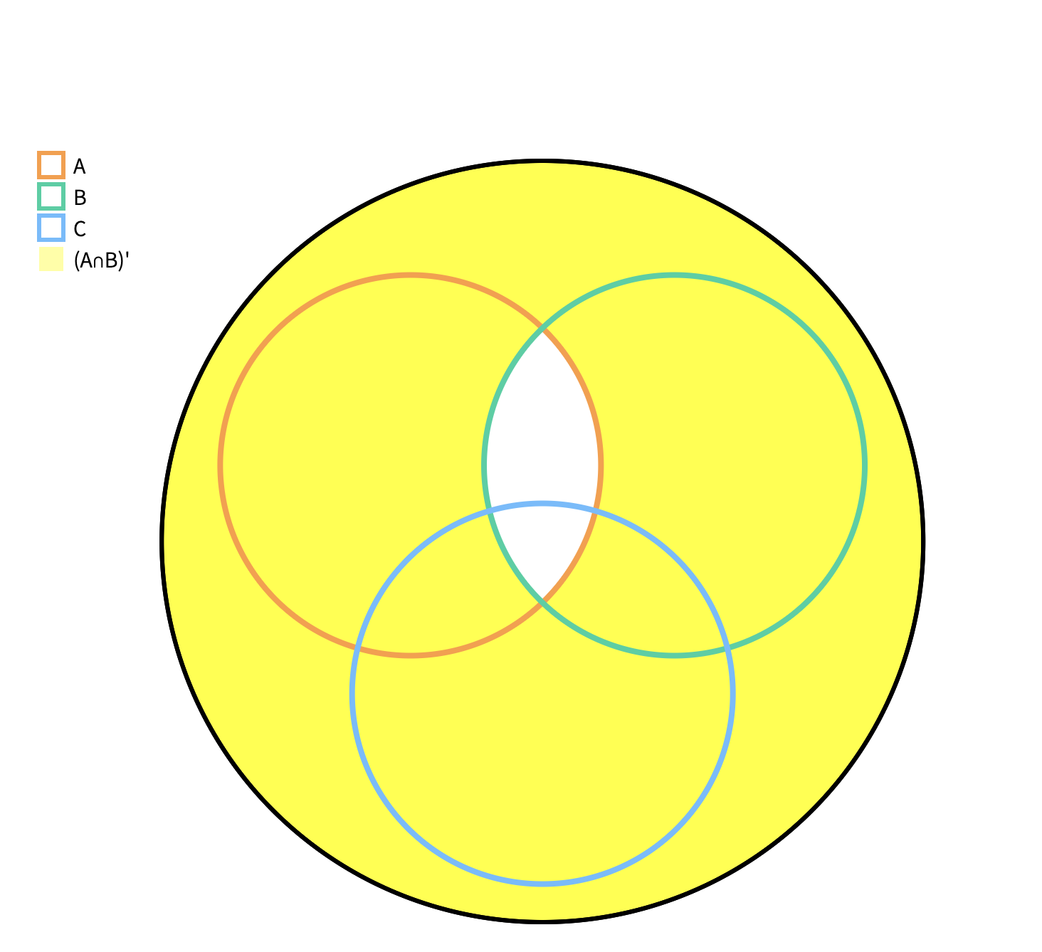
Set theory

pretty easy this diagrams explains all of it

Counting (permutation and combinations)

permutations: a permutation is an arrangement of items where the order matters. the formula for calculating the number of permutations of r items chosen from a set of n items is: p(n, r) or ₙpᵣ = n! / (n - r)! where:
- n! (n factorial) is the product of all positive integers up to n (e.g., 5! = 5 * 4 * 3 * 2 * 1)
- n is the total number of items in the set
- r is the number of items you’re choosing and arranging
combinations: a combination is a selection of items where the order does not matter. the formula for calculating the number of combinations of r items chosen from a set of n items is: c(n, r) or ₙcᵣ = n! / (r! * (n - r)!) where:
- n! (n factorial) is the product of all positive integers up to n
- n is the total number of items in the set
- r is the number of items you’re choosing

Conditional probability

this is when the probably of an event depends on the probability of another event

formula is : p(a|b) = p(a and b) / p(b) where p (a and b) are calculated using p(a) x p(b)

this gives us a final probability of a task when we have prev conditions

a real-life example: drawing cards

let’s consider a standard deck of 52 playing cards. we’re going to draw two cards without replacement (meaning we don’t put the first card back into the deck before drawing the second).

event a: the second card drawn is a heart.
event b: the first card drawn is a heart.

we want to find the conditional probability of the second card being a heart, given that the first card was a heart, or p(a|b).

probability of event b (the first card is a heart):
there are 13 hearts in a standard 52-card deck.
p(b) = 13 / 52 = 1 / 4
probability of both event a and event b (first card is a heart, and second is also a heart):
- probability that the first card is a heart is 13 / 52.
- given that the first card is a heart, there are now only 12 hearts left and 51 cards total.
- probability the second card is also a heart is 12 / 51
- therefore, p(a and b) = (13 / 52) * (12 / 51) = 1 / 17
applying the conditional probability formula: p(a|b) = p(a and b) / p(b) = (1 / 17) / (1 / 4) to divide a fraction, you multiply by the reciprocal:

p(a|b) = (1 / 17) * (4 / 1) = 4 / 17

therefore, the probability that the second card is a heart, given that the first card is a heart, is 4/17, which is approximately 0.235

random variable

a random variable is a variable whose value is a numerical outcome of a random phenomenon. in simpler terms, it’s a way to see how likely different outcomes are. so the a deck of 52 cards each card can have a number 1-52 or the 4 sets can have a number each. its technically not the sample set itself but the outcome number

probability distributions

there are two types of probability distributions

discrete
continous

discrete distributions

a discrete random variable can only take on a finite number of values or a countably infinite number of values. think of these as values you can count with whole numbers. examples include: the number of heads in 3 coin flips, the number of cars crossing a bridge in an hour, or the number of defects in a batch of items.

probability mass function (pmf): this is the function that describes the probability associated with each possible value of the discrete random variable, x.
the pmf is denoted by p(x), and it satisfies the following properties:
- 0 ≤ p(x) ≤ 1 (all probabilities must be between 0 and 1, inclusive).
- ∑ p(x) = 1 (the sum of all probabilities over all possible values of x must be equal to 1).

continous distribution

a continuous random variable can take any value within a given range or interval. think of these as values you measure, like height, weight, temperature, or time. they could be fractional. it can take on infinitely many values. the number doesn’t have to be an arbitrary whole one it can be a fraction or multiple outputs - probability density function (pdf): this is the function that describes the relative probability of a continuous random variable falling within a particular interval.

the pdf is denoted by f(x), and it has the following properties:
- f(x) ≥ 0 for all x (the pdf is always non-negative).
- ∫ f(x) dx = 1 (the area under the curve of the pdf over all possible values is equal to 1).
- note: the actual probability of a continuous random variable exactly matching one specific value is 0, we can only find probability for a range. you need to integrate the probability density function to get the probability.

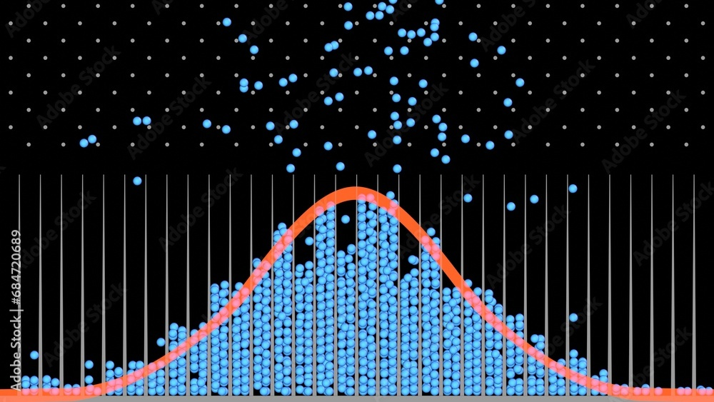
central limit theorem

probably the most fascinating thing in all of probability (lol) the bell curve it shows everywhere this is the true manifestation of averages this is a better explaination just watch this https://www.youtube.com/watch?v=zeJD6dqJ5lo&t=747s now this is a weird topic actually everytime you work with probabilites you can map it to a general distribution but the tricky part is relating to it now in a die roll where the distribution is already the bell curve (mean of sample is technically a bell curve) we map it to the addition of all the random variables (outcome of the die roll) over how many time you rolled the die (sample size) that is also a bell curve here is a more detailed explaination by chatgpt

Step 1: Define the Problem

Single Dice Roll:
- Outcomes: X∈{1,2,3,4,5,6}X \in {1, 2, 3, 4, 5, 6}X∈{1,2,3,4,5,6}.
- Probability of each outcome: P(X=k)=16P(X = k) = \frac{1}{6}P(X=k)=61 for k∈{1,2,3,4,5,6}k \in {1, 2, 3, 4, 5, 6}k∈{1,2,3,4,5,6}.
- Mean of a single dice roll (μ\muμ): μ=E[X]=1+2+3+4+5+66=3.5\mu = \mathbb{E}[X] = \frac{1 + 2 + 3 + 4 + 5 + 6}{6} = 3.5μ=E[X]=61+2+3+4+5+6=3.5
- Variance of a single dice roll (σ2\sigma^2σ2): σ2=E[(X−μ)2]=16∑k=16(k−3.5)2=2.92\sigma^2 = \mathbb{E}[(X - \mu)^2] = \frac{1}{6} \sum_{k=1}^{6} (k - 3.5)^2 = 2.92σ2=E[(X−μ)2]=61k=1∑6(k−3.5)2=2.92
Sum of nnn Rolls:
- Let SnS_nSn be the sum of nnn independent dice rolls: Sn=X1+X2+⋯+XnS_n = X_1 + X_2 + \dots + X_nSn=X1+X2+⋯+Xn
- Mean of SnS_nSn: E[Sn]=nμ\mathbb{E}[S_n] = n \muE[Sn]=nμ.
- Variance of SnS_nSn: Var(Sn)=nσ2\text{Var}(S_n) = n \sigma^2Var(Sn)=nσ2 (since dice rolls are independent).
Sample Mean:
- Let Xˉn\bar{X}_nXˉn be the sample mean of nnn rolls: Xˉn=Snn.\bar{X}_n = \frac{S_n}{n}.Xˉn=nSn.
- Mean of Xˉn\bar{X}_nXˉn: E[Xˉn]=E[Sn]n=μ.\mathbb{E}[\bar{X}_n] = \frac{\mathbb{E}[S_n]}{n} = \mu.E[Xˉn]=nE[Sn]=μ.
- Variance of Xˉn\bar{X}_nXˉn: Var(Xˉn)=Var(Sn)n2=nσ2n2=σ2n.\text{Var}(\bar{X}_n) = \frac{\text{Var}(S_n)}{n^2} = \frac{n \sigma^2}{n^2} = \frac{\sigma^2}{n}.Var(Xˉn)=n2Var(Sn)=n2nσ2=nσ2.

the main point is the sample you are taking the more the sample the better it fits into the bell curve

bayes’ theorum

this is an incredible stats subfield basically based on previous data and its probability you can figure out the properties of your own caluclated probabilty (this sounds stray from the original defintition but will make more sense when you read the doctor’s positive result experiment) Suppose that on your most recent visit to the doctor’s office, you decide to get tested for a rare disease. If you are unlucky enough to receive a positive result, the logical next question is, “Given the test result, what is the probability that I actually have this disease?” (Medical tests are, after all, not perfectly accurate.) Bayes’ Theorem tells us exactly how to compute this probability: p(a|b) = [p(b|a) * p(a)] / p(b)

where:

p(a|b): the posterior probability – the probability of hypothesis a being true given the evidence b. this is what we want to calculate.
p(b|a): the likelihood – the probability of seeing the evidence b given that the hypothesis a is true.
p(a): the prior probability – our initial belief in the probability of hypothesis a being true before seeing any evidence.
p(b): the evidence – the probability of observing the evidence b, regardless of the hypothesis. this can be computed by considering all ways b could happen.

so in this scenario hypothesis a: a patient has the disease (we want to know p(a)) evidence b: the patient tested positive on a diagnostic test. (we have this evidence). prior probability (p(a)): the probability that a random person has the disease is 0.01 (1% of people have it). this is the base probability of someone having the disease. likelihood (p(b|a)): the probability of a patient testing positive if they do have the disease is 0.95 (the test is 95% accurate for people with the disease). this is the true positive rate. probability of evidence (p(b)): we will calculate this. we will need to consider both people that have the disease and don’t have the disease: - p(b | a) = 0.95. we already know this value from above. the probability of someone with the disease testing positive.

- p(a) = 0.01 the probability of someone having the disease (given).
    
- p(not a) = 0.99 the probability of someone not having the disease (given).
    
- p(b | not a) = 0.05. the probability of someone without the disease testing positive (5% false positive).
    
    - p(b) = p(b|a)p(a) + p(b|not a)p(not a) = (0.95 * 0.01) + (0.05 * 0.99) = 0.0095 + 0.0495 = 0.059

minor detour to understand the law of total probability skip if you already know

the law of total probability

the law of total probability is a fundamental concept in probability theory that allows you to calculate the probability of an event by considering all the possible ways it can occur, given a set of mutually exclusive and exhaustive events.

mutually exclusive events: these are events that cannot happen at the same time (e.g., a patient either has the disease or doesn’t, but not both simultaneously).
exhaustive events: these are events that cover all possible outcomes (e.g., for disease, the patient either has it or doesn’t; there’s no other option).

applying the law to our example

in our medical diagnosis example:

event b: the patient tests positive.
event a: the patient has the disease.
event not a: the patient does not have the disease.

note: ‘a’ and ‘not a’ are mutually exclusive and collectively exhaustive. they cover all cases.

the law of total probability says that the probability of the patient testing positive (event b) can occur in one of two ways:

testing positive, given they have the disease: this is represented by p(b|a) * p(a). it’s the probability of a positive test, given the patient has the disease, times the probability the patient has the disease.
testing positive, given they do not have the disease: this is represented by p(b|not a) * p(not a). it’s the probability of a positive test, given the patient does not have the disease, times the probability the patient does not have the disease.

to find the total probability of testing positive, p(b), you sum up the probabilities of these two mutually exclusive ways of getting a positive test:

p(b) = p(b|a)p(a) + p(b|not a)p(not a)

why this works:

this formula comes from applying some basic rules of probability:

the multiplication rule: the probability of two events a and b both occurring is p(a and b) = p(b|a) * p(a). so, p(b|a)p(a) is the probability that the patient has the disease and tests positive.
partitioning the event space: we are partitioning the event of testing positive (event b) into two mutually exclusive groups: those that have the disease and test positive, and those that don’t have the disease but still test positive. therefore all of the ways of getting ‘b’ are accounted for, there are no others.
addition rule: since the two ways of getting a positive test are mutually exclusive (you can’t both have the disease and not have the disease), we add the probabilities of each event occurring. this is because the probability of getting a positive is composed of the probability of getting a true positive (if you have the disease) or getting a false positive (if you don’t).

in our numerical example:

p(b) = p(b|a)p(a) + p(b|not a)p(not a)

p(b) = (0.95 * 0.01) + (0.05 * 0.99) = 0.0095 + 0.0495 = 0.059

0.0095 represents the probability of a true positive result (a patient with the disease testing positive).
0.0495 represents the probability of a false positive result (a patient without the disease testing positive).

by adding these, we get 0.059, which is the probability that anyone tests positive regardless of whether they have the disease or not.

generalized form

the law of total probability can be generalized to any number of mutually exclusive and exhaustive events (a₁, a₂, a₃… aₙ):

p(b) = p(b|a₁)p(a₁) + p(b|a₂)p(a₂) + p(b|a₃)p(a₃) + … + p(b|aₙ)p(aₙ)

applying bayes’ theorem:

now we can calculate the posterior probability, p(a|b), the probability that a patient has the disease given that they tested positive:

p(a|b) = [p(b|a) * p(a)] / p(b)
p(a|b) = (0.95 * 0.01) / 0.059
p(a|b) = 0.0095 / 0.059
p(a|b) ≈ 0.161

which is crazy because wdym a test that is correct 95% of the time only has a porbabiltiy of being correct 16% when i am tested positive lol now this breaks a lot of intuition but think of it this way only 1 percent of the people have this disease is it more likely that you have it or that the test went wrong.

Links

links that might be usefull in learning concepts https://www.youtube.com/watch?v=zeJD6dqJ5lo&t=747s https://www.youtube.com/playlist?list=PLBh2i93oe2qswFOC98oSFc37-0f4S3D4z https://youtu.be/3jP4H0kjtng?si=cZ-9oJMVVrLtMjxT